6. LiDAR, Terrain, and 3D
2:00 - 3:00 p.m.
Lecture 15 min · Hands-on 35 min · Break 2:50 - 3:00
Learning goals
- Explain how COPC and EPT make billion-point LiDAR surveys viewable in a browser.
- Stream a USGS 3DEP point cloud for Reno and color it by elevation and classification.
- Tilt and rotate the camera, and turn on 3D terrain.
- Know when to reach for the Cesium globe or 3D Tiles.
Lecture (15 min)
Point clouds in the cloud
A LiDAR survey of a metro area easily holds billions of points. Two cloud-native layouts make it practical to view one over HTTP:
- COPC (Cloud-Optimized Point Cloud) is a single LAZ file whose points are arranged in an octree. A viewer reads the hierarchy first, then only the nodes that are visible at the current level of detail.
- EPT (Entwine Point Tile) stores the same kind of octree as many small
files listed by an
ept.json. The USGS publishes its entire 3DEP LiDAR program this way on Amazon S3, with more than 2,000 projects.
Both let the viewer stop at a point budget: it draws a representative sample of the survey at a regional view and fills in detail where you zoom.
ASPRS classification codes
Classified LiDAR assigns each point a class. The common ones:
| Code | Class | Code | Class |
|---|---|---|---|
| 1 | Unclassified | 6 | Building |
| 2 | Ground | 7 | Low noise |
| 3 | Low vegetation | 9 | Water |
| 4 | Medium vegetation | 17 | Bridge deck |
| 5 | High vegetation | 18 | High noise |
Ground points (class 2) build bare-earth DEMs like the one in Sections 3 and 5. The USGS 3DEP DEM is derived from exactly these surveys.
3D in GeoLibre
- Pitch and bearing tilt and rotate the 2D map (MapLibre supports pitch up to 85°).
- Terrain (Controls → Terrain) drapes the basemap and layers over global elevation tiles.
- 3D extrusion in the Style panel raises building footprints by a height attribute, and the Liberty 3D basemap includes 3D buildings.
- Add data → 3D layers adds LiDAR, Gaussian splats, OGC 3D Tiles, glTF models, and Cesium ion assets.
- View → Rendering engine → Cesium switches to a full 3D globe.
Hands-on (35 min)
Start a new project named NGIS 2026 - 6 LiDAR and 3D with the
Liberty 3D basemap.
Exercise 6.1: Stream the USGS Reno-Carson survey (10 min)
- Choose Add data → LiDAR layer.
-
In Load COPC or EPT from URL, paste the USGS 3DEP Reno-Carson 2017 (QL1) survey and click Load:
https://s3-us-west-2.amazonaws.com/usgs-lidar-public/USGS_LPC_NV_Reno_Carson_QL1_2017_LAS_2018/ept.json -
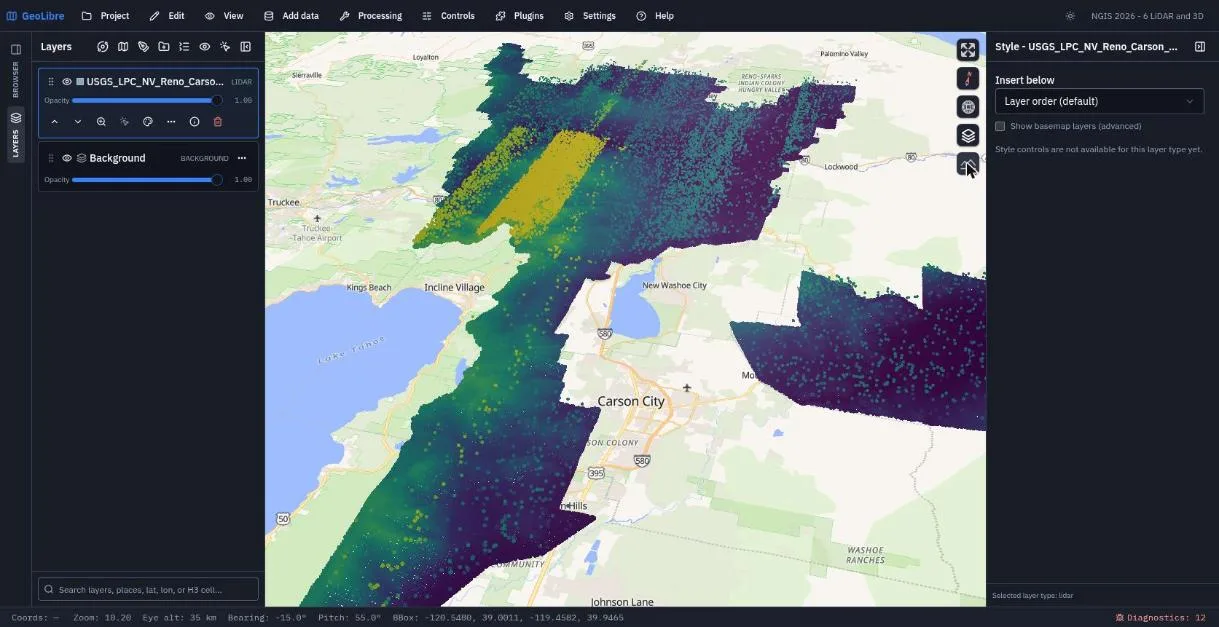
The map zooms to the survey, which runs from north of Reno past Carson City to the east shore of Lake Tahoe. The points are colored by Elevation with the Viridis colormap.
- Note the size: the survey holds roughly 20 billion points. The viewer draws a sample within its point budget and refines it as you zoom.
Find a survey near you
The USGS 3DEP LiDAR boundaries map lists every
EPT on Amazon S3. Swap in any ept.json URL. A smaller QL2 survey of the
same area is USGS_LPC_NV_Reno_Carson_QL2_2017_LAS_2018.
Exercise 6.2: Tilt the camera and add terrain (8 min)
- Choose View → Set view... and enter:
Longitude
-119.80, Latitude39.25, Zoom10.2, Pitch55, Bearing-15. Click Go. - The Carson Range and the Sierra front now rise toward Lake Tahoe.
- Choose Controls → Terrain, then click the mountain button that appears in the map controls to turn 3D terrain on.
- Tilt and rotate by hand: drag with the right mouse button (or
Ctrl+drag) to change pitch and bearing. Click the compass to reset north.
Exercise 6.3: Color by classification (7 min)
- Open Add data → LiDAR layer again to bring back the LiDAR panel.
- Under Styling, set Color By to Classification. Ground turns brown, buildings magenta, and water blue.
- Zoom in to downtown Reno. Watch the point budget at work: at street level the sample thins out, because a 20-billion-point survey cannot all be in memory at once.
- Try Intensity, then set Color By back to Elevation.
Exercise 6.4: Full detail on a small cloud (10 min)
Regional surveys show the big picture; a small COPC shows full detail.
- In the LiDAR panel, open Sample data and pick Autzen (a classified COPC of the Autzen Stadium area in Eugene, Oregon).
- Color it by Classification and tilt the view to see trees, buildings, and the stadium bowl in 3D.
- Tick Enable point picking and click points to read their attributes.
- Remove the Autzen layer before saving, so the project stays on Reno.
Save the project.
Check your work
The finished project restores the Reno-Carson survey, the pitched camera, and 3D terrain.
Going further
- Plugins → Web services → USGS LiDAR clips a 3DEP point cloud to an area you draw and saves it as COPC.
- Plugins → Point cloud annotation selects points with a box or lasso and assigns ASPRS classes.
- Plugins → Elevation profile draws a terrain profile along a line.
- Switch to View → Rendering engine → Cesium for a 3D globe.
- Read Rendering Engines and Point Cloud Annotation.
Break: 2:50 - 3:00. Next: 7. Plugins and AI