4. STAC Catalogs and OGC Web Services
11:00 a.m. - 12:00 p.m.
Lecture 20 min · Hands-on 30 min · Break 11:50 - 12:00, then lunch until 1:00
Learning goals
- Describe how a STAC catalog organizes collections, items, and assets.
- Search a STAC API by area, date, and cloud cover, and add an imagery asset to the map.
- Add a Web Map Service (WMS) layer and an OGC API - Features layer.
- Tell a rendered map service apart from a feature service.
Lecture (20 min)
STAC: a catalog of files
The SpatioTemporal Asset Catalog (STAC) specification describes geospatial data as JSON:
- A catalog or collection groups related data, for example
sentinel-2-l2a. - An item is one footprint at one time, such as one Sentinel-2 scene, with
properties like
datetimeandeo:cloud_cover. - An asset is a file of that item: a true-color COG (
visual), a single band (red,nir), a cloud mask, or metadata.
A STAC API adds search (/search) by bounding box, date range,
collection, and property filters. A static catalog is just linked JSON
files on a web server. STAC Index lists hundreds of
public catalogs. Because the assets are usually COGs, a STAC search leads
straight to cloud-native reads.
OGC services: maps versus features
| Service | Returns | You get |
|---|---|---|
| WMS (Web Map Service) | Rendered images | A picture of the data; attributes only through GetFeatureInfo |
| WMTS / XYZ tiles | Pre-rendered image tiles | Fast display |
| WFS (Web Feature Service) | Features as GML or GeoJSON | Geometry and attributes |
| OGC API - Features | GeoJSON over a REST/JSON API | Geometry and attributes, paged |
| WCS (Web Coverage Service) | Raw raster values | Numbers you can analyze |
Rule of thumb: use a map service when you need a reference layer to look at, and a feature or coverage service when you need data to analyze.
Hands-on (30 min)
Start a new project named NGIS 2026 - 4 STAC and web services. Search for
Lake Tahoe in the search box and pick Lake Tahoe, Placer County,
California, then zoom out until the whole lake and Reno are in view (zoom
about 9). Clear the search box to remove the pin.
Exercise 4.1: Search Sentinel-2 with STAC (17 min)
- Choose Plugins → Web services → STAC catalogs. The panel docks on the right.
-
In STAC catalog or API URL, enter Element 84's Earth Search and click Connect:
https://earth-search.aws.element84.com/v1 -
In the collection list, select Sentinel-2 Level-2A.
- Keep Limit search to the current map extent ticked.
- Set Start date to
07/01/2025and End date to08/31/2025. -
In Additional search parameters, enter a cloud-cover filter and a sort order:
{"query": {"eo:cloud_cover": {"lt": 5}}, "sortby": [{"field": "properties.datetime", "direction": "desc"}]} -
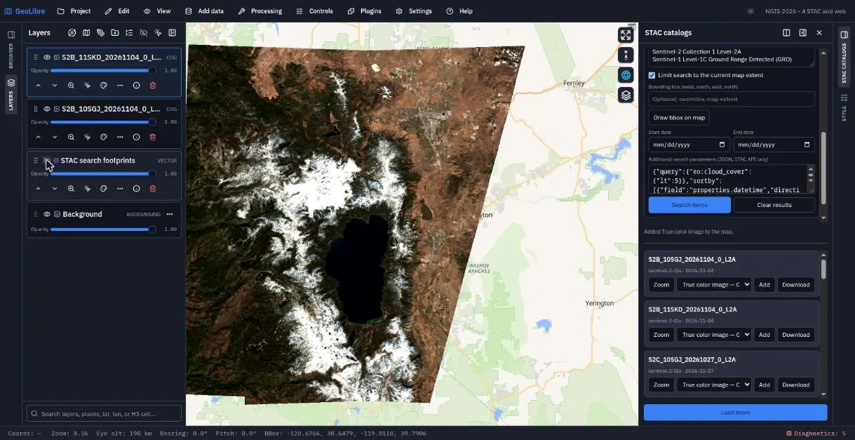
Click Search items. Footprints appear on the map, and the list shows matching scenes with their dates.
- Lake Tahoe straddles two Sentinel-2 tiles,
10SGJand11SKD. For a scene from each tile on the same date, pick True color image — COG in the asset menu and click Add. - Hide the
STAC search footprintslayer and compare the scenes with the basemap.
Try other assets
The asset menu lists every band. Add nir (near infrared) and compare
vegetation with the true-color image. Raster rendering options in the
panel set bands, colormap, min/max, and NoData for assets you add next.
Exercise 4.2: A WMS layer (5 min)
- Close the STAC panel. Choose Add data → WMS layer.
- Layer name:
USGS hydrography (WMS). -
Service URL:
https://basemap.nationalmap.gov/arcgis/services/USGSHydroCached/MapServer/WMSServer -
Click Retrieve layers. The service offers one layer,
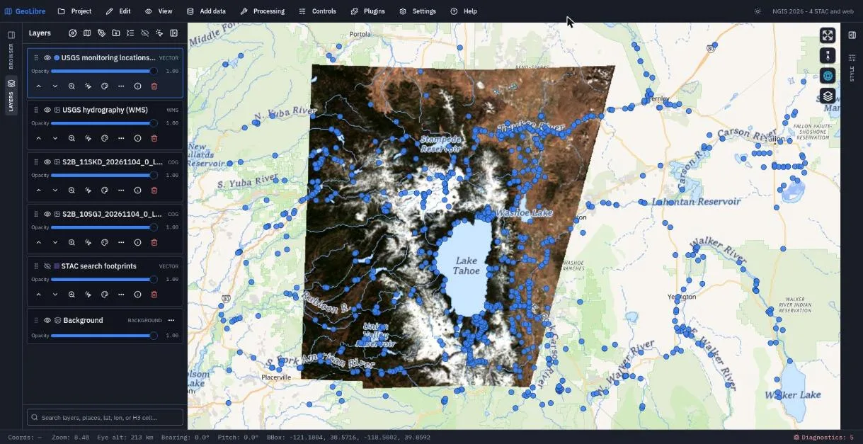
0. Click Add layer. - Streams, rivers, and lakes from the National Hydrography Dataset draw over the imagery. Try identifying a river: a WMS returns pixels, so attributes come only from GetFeatureInfo where the server supports it.
Exercise 4.3: OGC API - Features (8 min)
- Choose Add data → OGC API - Features.
- Layer name:
USGS monitoring locations (OGC API). -
Service URL:
https://api.waterdata.usgs.gov/ogcapi/v0 -
Click Retrieve collections. The USGS Water Data API lists 39 collections. Type
monitoring-locationsin Collection. - Leave Max features at 1000 and click Use view to fill the Bounding box with the current map extent.
- Click Add layer. Stream gages, wells, and other sites appear as points.
- Open the attribute table for the new layer. These are real features with attributes such as site names and types, unlike the WMS picture.
Save the project.
Check your work
Going further
- Open a STAC collection directly with a link:
https://web.geolibre.app/?stac=https://earth-search.aws.element84.com/v1/collections/naip - Plugins → Web services has ready-made browsers for USGS National Map, USGS 3DEP, FEMA NFHL, NASA Earthdata, Planet Open Data, Sentinel-2 Explorer, and dozens more.
- Add data → ArcGIS layer reads ArcGIS FeatureServer, MapServer, ImageServer, and VectorTileServer URLs.
- Read Web Services and Adding Data.
Break: 11:50 - 12:00. Lunch: 12:00 - 1:00. Next: 5. Spatial Analysis