2. Accessing Cloud-Hosted Vector Data
9:00 - 10:00 a.m.
Lecture 15 min · Hands-on 35 min · Break 9:50 - 10:00
Learning goals
- Load vector data from public URLs: GeoJSON, CSV with coordinates, and FlatGeobuf.
- Style a layer with single, graduated, and categorized symbology.
- Add labels and a legend.
- Explore features in the attribute table.
Lecture (15 min)
Where cloud-hosted vector data lives
Public vector data is published in many places: government open-data portals, GitHub repositories, object storage buckets (Amazon S3, Source Cooperative, Hugging Face), and APIs. If a file has a public HTTPS URL and the server sends cross-origin (CORS) headers, GeoLibre can read it directly in the browser.
| Format | Strength | Weakness |
|---|---|---|
| GeoJSON | Human-readable, universal | Large, must be read whole |
| CSV with lon/lat columns | Easy to produce from any spreadsheet or API | Points only, no CRS metadata |
| Shapefile (zipped) | Everywhere in legacy GIS | Many sidecar files, 2 GB limit, 10-character field names |
| GeoPackage | One SQLite file, many layers | Not designed for partial reads over HTTP |
| FlatGeobuf | Streams features, has a spatial index | Less common than GeoJSON |
| GeoParquet | Compressed, columnar, fast to query | Binary, needs a Parquet reader |
GeoLibre's Add data → Vector layer reads all of these. In the browser, formats MapLibre cannot draw natively are converted on the fly by DuckDB-WASM Spatial. Vector data is reprojected to WGS84 (EPSG:4326) on load, using the CRS stored in the file. If a layer lands in the wrong place or not at all, its CRS is probably missing or not an EPSG code: convert it to WGS84 first, or set Source CRS override in the Add Vector Layer panel.
Symbology in one slide
- Single symbology: one color for every feature.
- Graduated: a numeric field split into classes (equal interval, quantile, natural breaks, and others) and mapped to a color ramp. Use it for magnitudes, rates, and densities.
- Categorized: one color per distinct value. Use it for types and classes.
- Rule-based and Advanced expression: full control with MapLibre expressions.
Quantile classes put the same number of features in each class, which works well for skewed data such as earthquake magnitudes, where most events are small.
Hands-on (35 min)
Start a new project: Project → New..., name it
NGIS 2026 - 2 Vector data and styling, keep the Liberty basemap, and click
Create.
Exercise 2.1: Load the counties (3 min)
-
Add data → Vector layer, paste the URL below, and click Load:
https://assets.geolibre.app/data/workshops/ngis-2026/nv_counties.geojson -
Also load the landmarks:
https://assets.geolibre.app/data/workshops/ngis-2026/reno_sites.geojson -
Close the panel and rename the layers
Nevada countiesandReno-Tahoe sites(double-click the name).
Exercise 2.2: Load earthquakes from a CSV (5 min)
The USGS earthquake catalog exports CSV files with latitude and longitude
columns. This extract holds 8,031 M2.5+ earthquakes from 2016 through 2025.
- Add data → Delimited text layer.
- Layer name:
Nevada earthquakes. -
Source type: Delimited text URL. Paste:
https://assets.geolibre.app/data/workshops/ngis-2026/nv_earthquakes.csv -
Click Retrieve columns. The dialog reports Retrieved 8 columns and picks
longitudeandlatitudeautomatically. - Leave Coordinate system blank (the coordinates are already WGS84) and click Add layer.
Exercise 2.3: Graduated symbols by magnitude (8 min)
- Click the palette icon on the
Nevada earthquakesrow to open the Style panel. - Set Style type to Graduated.
- Attribute:
mag. Classes: 5. Scheme: Quantile. - Click the Colormap button and choose Plasma.
- Click Apply style type. The stops read about 2.5, 2.6, 2.72, 2.9, and 3.28: most events are barely above the M2.5 cutoff.
- Try Scheme: Equal interval and apply again. Most points fall into the first class. Which scheme tells the better story? Switch back to Quantile.
Style suggestions
The Style panel also offers one-click suggestions based on the data, such as Categorize by magType, Graduate by depth, and Heatmap. Try Heatmap, then switch back.
Exercise 2.4: Outline counties and label them (6 min)
- Open the Style panel for
Nevada counties. - Next to Fill color, tick Transparent. Set Stroke width to
2. - Scroll to Labels, tick Show labels, and set Label field to
NAME. County names appear at their centroids.
Exercise 2.5: Legend and attribute table (8 min)
- Choose Controls → Legend. The legend lists each layer and the five magnitude classes.
- On the
Nevada earthquakesrow, open Layer actions (⋯) → Open attribute table. The table docks below the map and reports 8031 features. - Tick Zoom to selection in the table toolbar, sort by
mag, and click the strongest event (M7.1, Ridgecrest, California, July 2019) to find it on the map. - Explore the table toolbar: field statistics, charts, and Select by expression.
- Close the table and save the project (Project → Save).
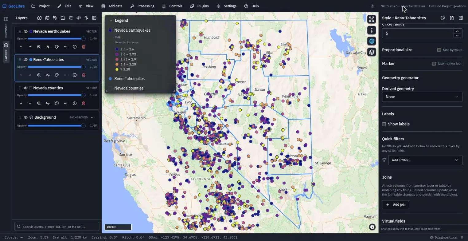
Exercise 2.6: FlatGeobuf (5 min)
FlatGeobuf streams features in order and carries a spatial index, so it loads faster than GeoJSON for large layers.
-
Add data → FlatGeobuf layer. Paste the 3,235 US counties into Vector URL (the Format reads FlatGeobuf) and click Add Layer:
https://assets.geolibre.app/data/workshops/ngis-2026/us_counties.fgb -
The layer list tags it
FLATGEOBUF. Compare how long it takes with the 17-county GeoJSON, then remove the layer (trash icon) to keep this project focused on Nevada.
Check your work
Why this project file is larger
A CSV layer is converted to points when it loads, and the converted features are embedded in the saved project, so this project is about 2 MB. Layers loaded from GeoJSON, GeoParquet, or tiles store only their URL.
Going further
- Add data → Administrative boundaries adds geoBoundaries polygons for any country.
- Plugins → Web services → US state GIS browses every state's open-data portal, including Nevada's.
- Read Styling Layers and Attribute Table.
Break: 9:50 - 10:00. Next: 3. Cloud-Native Formats