3. Cloud-Native Formats: COG, GeoParquet, PMTiles, and Zarr
10:00 - 11:00 a.m.
Lecture 20 min · Hands-on 30 min · Break 10:50 - 11:00
Learning goals
- Explain how each cloud-native format lets a client read only what it needs.
- Load and style a Cloud-Optimized GeoTIFF (COG).
- Stream a GeoParquet file without copying it into memory.
- Load a PMTiles archive and a Zarr data cube.
- Choose the right format for a given task.
Lecture (20 min)
The common trick: a small index, read first
Every cloud-native format does the same two things: it keeps an index (metadata) that a client can read with one small request, and it chunks the data so each request returns a useful piece. Where the index lives differs: at the start of a COG, at the end of a GeoParquet file (the footer), and in separate small files for Zarr and EPT, whose chunks are separate objects fetched by key rather than byte ranges within one file.
Every format needs a host that sends CORS headers. The single-file formats
(COG, GeoParquet, FlatGeobuf, PMTiles, COPC) also need HTTP Range support:
if a server ignores Range, a reader either falls back to downloading the
whole file or fails outright (the PMTiles reader rejects it). EPT and
unsharded Zarr fetch each chunk as its own object, so they need no range
support; sharded Zarr v3 packs many chunks into one object and reads them
with ranges again. Object
stores such as S3, GitHub Pages, and Source Cooperative support both.
| Format | Data type | Index | Chunk | Typical use |
|---|---|---|---|---|
| COG (Cloud-Optimized GeoTIFF) | Raster | TIFF header with tile offsets, plus overviews (reduced-resolution copies) | 256 or 512 px tiles | Imagery, elevation, land cover |
| GeoParquet | Vector table | Parquet footer: schema, row groups, column statistics, bounding boxes | Row group × column | Large tables to filter, aggregate, and join |
| FlatGeobuf | Vector features | Packed Hilbert R-tree | Feature | Streaming features by bounding box |
| PMTiles | Pre-rendered vector or raster tiles | Directory of tile offsets | One map tile (z/x/y) | Basemaps and fast cartographic display |
| Zarr | N-dimensional arrays | .zmetadata or zarr.json |
Array chunk (e.g. time × lat × lon) | Climate, weather, ocean model output |
| COPC / EPT | Point clouds | Octree hierarchy | Octree node | LiDAR (Section 6) |
A COG viewed at a small scale reads only an overview, a few hundred kilobytes, even if the full-resolution file is gigabytes. A GeoParquet query reads the footer, skips row groups whose bounding boxes miss the area of interest, and reads only the columns the query needs.
Which format when?
- Display a large raster: COG.
- Analyze a large table with SQL: GeoParquet.
- Pan around a big vector layer quickly at every zoom: PMTiles (the geometry is simplified per zoom level, so it is for display, not analysis).
- Slice a variable through time or depth: Zarr.
How the workshop data was made
The county files in the workshop bucket all came from one Census counties shapefile, and the elevation COG from four USGS 3DEP tiles, converted with standard open tools:
ogr2ogr -f FlatGeobuf us_counties.fgb cb_2023_us_county_500k.shp -t_srs EPSG:4326
ogr2ogr -f Parquet us_counties.parquet us_counties.fgb \
  -lco COMPRESSION=ZSTD -lco SORT_BY_BBOX=YES -lco WRITE_COVERING_BBOX=YES \
  -lco ROW_GROUP_SIZE=256
ogr2ogr -f PMTiles us_counties.pmtiles us_counties.fgb -dsco MAXZOOM=10
gdalwarp -of COG -co COMPRESS=DEFLATE -co OVERVIEWS=AUTO dem.vrt reno_tahoe_dem.tif
GeoLibre can do the same conversions in the browser with Processing → GeoLibre toolbox → Conversion (Vector to GeoParquet, Vector to FlatGeobuf, Vector to PMTiles, Raster to COG).
Hands-on (30 min)
Start a new project: Project → New..., name it
NGIS 2026 - 3 Cloud-native formats, pick the Positron basemap, and click
Create.
Exercise 3.1: A Cloud-Optimized GeoTIFF (8 min)
- Add data → Raster layer. Leave the rendering engine at cog-tiler-wasm (WASM).
-
Paste the URL and click Load:
https://assets.geolibre.app/data/workshops/ngis-2026/reno_tahoe_dem.tif -
The map zooms to the Reno-Tahoe area. Close the Add Raster Layer panel.
- In the Style panel, open Color ramp and choose terrain. The histogram below the ramp shows the elevation range, about 1,300 to 3,300 m.
- The DEM is 2520 × 3240 pixels and 22 MB, yet it appeared almost instantly: the browser fetched only the overview tiles it needed for the current view.
- Use Inspect pixel values on the layer row and click Mount Rose (northeast of Lake Tahoe) to read its elevation.
Discussion
Lake Tahoe shows as a flat area at about 1,897 m. Why does the terrain ramp paint some low valleys blue as if they were water?
Exercise 3.2: Stream a GeoParquet file (8 min)
- Add data → GeoParquet layer.
-
Tick Stream GeoParquet (no copy). Paste the URL and click Load:
https://assets.geolibre.app/data/workshops/ngis-2026/us_counties.parquet -
The panel lists the layer as
geoparquet · 3.2k ft · geojson · stream. The file is read in place with HTTP range requests instead of being copied into memory. - The map zooms out to the full extent, which spans Guam to the Aleutians.
Type
Nevadain the search box and pick Nevada, United States, then zoom out a few steps. - Open View → Set view... to type an exact camera if you overshoot.
Streaming or not?
Streaming suits large, spatially sorted files. This file was written with
SORT_BY_BBOX and 256-row groups (14 in all), so nearby counties sit in
the same row groups and a reader can skip the rest. For small
files, leave streaming off: you get the full Style panel and the attribute
table.
Exercise 3.3: PMTiles (7 min)
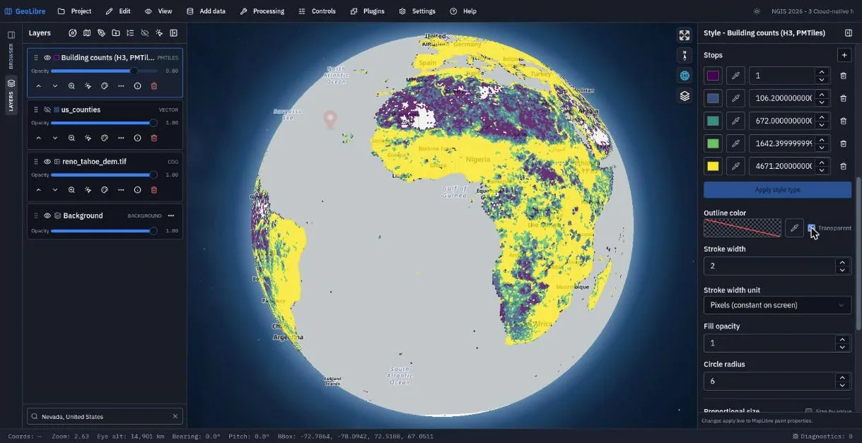
- Hide the
us_countieslayer (eye icon). -
Add data → PMTiles layer. Paste:
https://data.source.coop/giswqs/opengeos/building_count_h3.pmtiles -
Click Fetch. The dialog finds one source layer,
data. Set Layer Name toBuilding counts (H3, PMTiles)and click Add Layer. - In the Style panel choose Style type: Graduated, Attribute: building_count, Scheme: Quantile, and click Apply style type. Under Outline color, tick Transparent.
- Zoom in and out. Each zoom level requests a handful of tiles from a single archive file, with no tile server involved.
Exercise 3.4: Zarr (7 min)
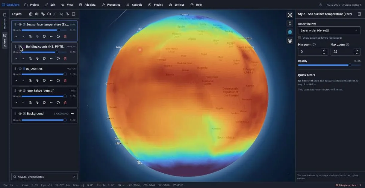
- Hide the PMTiles layer.
- Add data → Zarr layer. Open Load sample data... and pick the NOAA
monthly Sea surface temperature sample (OISST). The form fills in the URL, the
variable
sst, and a display range of -2 to 32 °C. - Tick Pickable (click to show pixel value), set Layer Name to
Sea surface temperature (Zarr), and click Add Layer. - Zoom out to a global view and click the ocean to read temperatures.
- Change Selector (JSON) to pick another time step, for example
{"time": 12}, and add it as a second layer. Toggle between them.
A 404 in Diagnostics is expected
The Zarr reader first checks for a Zarr v3 zarr.json. This store is Zarr
v2, so that check returns 404 and the reader falls back to .zmetadata.
The Diagnostics counter in the status bar records the 404; it is harmless.
Save the project.
Check your work
The finished project opens on the counties with the PMTiles and Zarr layers hidden. Toggle them on in the Layers panel.
Going further
- Open your browser's developer tools (F12), go to the Network tab, and pan
the COG. Look for
206 Partial Contentresponses: the request carries aRangeheader and the response a matchingContent-Rangeheader. - Convert a file of your own with Processing → GeoLibre toolbox → Conversion.
- Browse more cloud-native datasets with Plugins → Web services → Source Cooperative.
- Read Cloud-Native Data and Supported Data Formats.
Break: 10:50 - 11:00. Next: 4. STAC Catalogs and OGC Web Services