5. Spatial Analysis with SQL and Processing Tools
1:00 - 2:00 p.m.
Lecture 15 min · Hands-on 35 min · Break 1:50 - 2:00
Learning goals
- Query map layers and remote files with DuckDB spatial SQL in the browser.
- Run a spatial join and turn the result into a choropleth layer.
- Buffer features and count what falls inside each buffer.
- Derive a hillshade from an elevation model without any server.
Lecture (15 min)
Analysis in the browser
GeoLibre runs most analysis on your own machine:
| Engine | Where it runs | Used for |
|---|---|---|
| DuckDB-WASM Spatial | Browser | The SQL workspace, file conversion, GeoParquet reads |
| PGlite + PostGIS | Browser | PostGIS-flavored SQL over loaded layers |
| Turf.js | Browser | The Client engine of the vector tools |
| Pyodide (GeoPandas, Shapely) | Browser | The Python engine of the vector tools |
| Client raster tools | Browser | Hillshade, slope, aspect, raster calculator, reclassify, and more |
| WhiteboxTools (WebAssembly) | Browser | The Whitebox toolbox |
| Python sidecar (rasterio, GeoPandas) | Desktop app, or a self-hosted server | Heavier raster tools and projection-aware vector tools |
Spatial SQL in five lines
Every vector layer on the map is a table in the SQL workspace, with its
geometry in a column named geom. DuckDB's ST_* functions follow the same
conventions as PostGIS:
SELECT c.NAME, count(q.id) AS quakes
FROM nv_counties c
LEFT JOIN nv_earthquakes q ON ST_Within(q.geom, c.geom)
GROUP BY c.NAME;
A LEFT JOIN keeps counties with zero matches. ST_Within(point, polygon)
is the point-in-polygon test. The workspace can also read files by URL
(FROM 'https://.../file.parquet'), so you can query data you have not added
to the map.
Degrees are not meters
The layers are in WGS84 longitude and latitude. ST_Area and ST_Distance
on them return square degrees and degrees. For buffers, use the
Buffer tool, which takes kilometers.
Hands-on (35 min)
Start a new project named NGIS 2026 - 5 Spatial analysis. Use
Add data → Vector layer to load these three URLs (paste each and click
Load):
https://assets.geolibre.app/data/workshops/ngis-2026/nv_counties.geojson
https://assets.geolibre.app/data/workshops/ngis-2026/nv_earthquakes.parquet
https://assets.geolibre.app/data/workshops/ngis-2026/reno_sites.geojson
This time the earthquakes come from GeoParquet instead of CSV.
Exercise 5.1: Explore a table with SQL (5 min)
- Choose Processing → SQL workspace. It docks below the map, with the
engine set to DuckDB. The Queryable layers line lists
nv_counties,nv_earthquakes, andreno_sites. -
Replace the sample query with the one below and press
Ctrl+Enter(or click Run):DESCRIBE nv_earthquakes; -
Note the
geomcolumn of typeGEOMETRY('EPSG:4326'), and thattimearrived as a BIGINT (milliseconds since 1970). -
Find the ten strongest events:
SELECT place, mag, depth, epoch_ms(time) AS time
FROM nv_earthquakes
ORDER BY mag DESC
LIMIT 10;
The top event is the M7.1 Ridgecrest earthquake of July 6, 2019, which struck California, not Nevada. Second is the M6.5 Monte Cristo Range earthquake of May 15, 2020, in Nevada. Keep that in mind for the next exercise.
Exercise 5.2: Earthquakes per county (10 min)
-
Run the spatial join:
SELECT c.NAME AS county, count(q.id) AS quakes, round(max(q.mag), 1) AS max_mag, c.geom FROM nv_counties c LEFT JOIN nv_earthquakes q ON ST_Within(q.geom, c.geom) GROUP BY c.NAME, c.geom ORDER BY quakes DESC; -
The result has 17 rows. Esmeralda leads with 1,431 events and a maximum of M6.5: the May 15, 2020 Monte Cristo Range earthquake and its aftershocks. Mineral (430) and Washoe (221) follow.
- Type
Earthquakes per countyin the Layer name box above the results and click Add as layer. - Close the SQL workspace. In the Style panel for the new layer, choose Graduated, Attribute: quakes, Scheme: Quantile, colormap Reds, and click Apply style type.
- Hide
nv_earthquakesandnv_countiesto see the choropleth.
Discussion
The 17 county counts add up to 2,827, yet the layer holds 8,031 events. The other 5,204 fall outside Nevada, mostly in California. Which part of the query removed them?
Exercise 5.3: Buffer and count (10 min)
- Choose Processing → GeoLibre toolbox → Vector → Buffer.
- Input layer:
reno_sites. Distance:10. Units: Kilometers. Buffer side: Outside (grow). Engine: Client (Turf.js). - Click Run. The output reads Buffered 8 feature(s) by 10 kilometers
(outside), and a
Bufferlayer appears. -
Close the dialog, reopen Processing → SQL workspace (the new layer is queryable as
buffer), and count earthquakes within 10 km of each site:SELECT b.name, count(q.id) AS quakes_10km, round(max(q.mag), 1) AS max_mag FROM buffer b LEFT JOIN nv_earthquakes q ON ST_Intersects(q.geom, b.geom) GROUP BY b.name ORDER BY quakes_10km DESC; -
Mount Rose summit tops the list with 13 events. The workshop venue has none within 10 km in this decade.
Faster from the map
Right-click the map to run a buffer or a drive-time isochrone around the clicked point, or use Layer actions → Quick analysis on a layer.
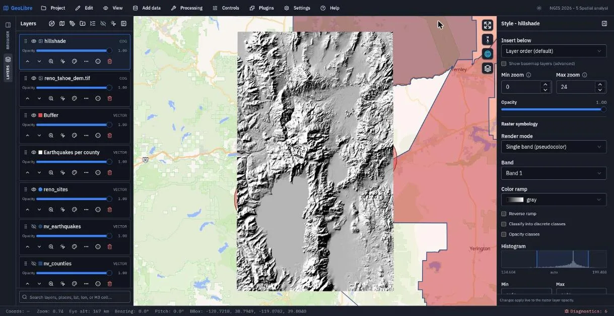
Exercise 5.4: Hillshade in the browser (10 min)
-
Add data → Raster layer, load the DEM, and close the panel:
https://assets.geolibre.app/data/workshops/ngis-2026/reno_tahoe_dem.tif -
Choose Processing → GeoLibre toolbox → Raster → Hillshade. You can also type
Hillshadeinto the search box at the top of the Processing menu. - Engine: Client (browser). Use a layer on the map:
reno_tahoe_dem.tif. Keep Azimuth 315, Altitude 45, Z factor 1. - Click Run. The log reports the raster size (2520 × 3240, 8.2 million pixels), then Added "hillshade.tif" to the map.
- Close the dialog. The new
hillshadelayer sits above the DEM. Set its opacity to about 0.5 and give the DEM a terrain color ramp to combine color and relief. Try Slope and Aspect too.
Computed layers are not saved
The hillshade lives only in browser memory. When you save, GeoLibre warns
that 1 local raster layer was not saved with the project. Click
Download GeoTIFF in the tool dialog to keep it, then host it and add it
by URL. The finished project points at a hosted copy,
reno_tahoe_hillshade.tif.
Save the project.
Check your work
Going further
- Write the per-county result to a file with Export GeoParquet in the SQL workspace.
- Switch the SQL workspace engine to PostGIS and run the same join. The
queries above are written for DuckDB; in PostgreSQL, quote mixed-case
columns (
c."NAME") and cast before rounding (round(max(q.mag)::numeric, 1)). - Chain tools into a reusable workflow with Processing → Model builder.
- Read SQL Workspace, Processing Tools, and Spatial SQL.
Break: 1:50 - 2:00. Next: 6. LiDAR, Terrain, and 3D