1. Introduction to GeoLibre and Cloud-Native GIS
8:00 - 9:00 a.m.
Lecture 20 min · Hands-on 30 min · Break 8:50 - 9:00
Learning goals
By the end of this section you will be able to:
- Explain what makes a GIS workflow "cloud-native" and why it matters.
- Find your way around the GeoLibre interface: menus, Layers panel, Style panel, status bar.
- Add data to a map from a URL, change the basemap, and inspect features.
- Save a map as a
.geolibre.jsonproject and reopen it from a link.
Lecture (20 min)
What is cloud-native GIS?
Traditional desktop GIS assumes that data lives on your disk: you download a zip, unpack it, convert it, and only then look at it. Cloud-native GIS flips that around. Data stays where it is published, in object storage such as Amazon S3 or a plain web server, and the client reads only the parts it needs over HTTP.
Three ideas make that work:
- HTTP range requests. A browser can ask a server for bytes 1,000 to 2,000 of a file instead of the whole file. Formats designed for this keep a small index that a client reads first (a COG header at the start of the file, a GeoParquet footer at the end, Zarr metadata in its own small file), then fetch the tiles or chunks for the current view. For GeoParquet, how much can be skipped depends on the file: spatially sorted row groups with bounding-box statistics, like the workshop files, let a reader skip most of them.
- Cloud-optimized formats. Cloud-Optimized GeoTIFF (COG) for rasters, GeoParquet and FlatGeobuf for vectors, PMTiles for tiled maps, Zarr for multidimensional arrays, and COPC or EPT for point clouds. Section 3 looks at each one.
- Catalogs and standard APIs. STAC catalogs describe what data exists and where its files are. OGC APIs (WMS, WFS, OGC API - Features) serve maps and features on demand. Section 4 covers both.
The result: you can explore a 400 MB elevation model, a national county layer, or a 20-billion-point LiDAR survey from a laptop browser in seconds, without a server of your own.
What is GeoLibre?
GeoLibre is a free, open-source (MIT) GIS application built for this model.
- One app, three ways to run it: the browser at
web.geolibre.app, a desktop app (Windows,
macOS, Linux), and a Jupyter widget through the
geolibrePython package. - Client-side by default: rendering (MapLibre GL JS and deck.gl), SQL (DuckDB-WASM), and many processing tools run in your browser. Your data leaves your machine only when you share or export it, or when you send a request to a remote AI provider through the AI Assistant. Searching places sends the search text to a geocoding service, and catalog and service searches send the map extent to that service.
- Projects are small JSON files: a
.geolibre.jsonproject stores layer sources, styles, the map view, and plugin state, so a whole map can be reopened from one URL. - Extensible: more than 70 built-in plugins (web-service catalogs, a time slider, LiDAR tools, AI segmentation) and an external plugin marketplace.
- Several rendering engines: MapLibre (the default), plus Mapbox, Cesium (3D globe), and ArcGIS under View → Rendering engine.
The interface
| Area | What it does |
|---|---|
| Top toolbar | Project, Edit, View, Add data, Processing, Controls, Plugins, Settings, Help menus. The project name sits on the right and can be edited in place |
| Layers panel (left) | Layer order, visibility, opacity, and per-layer buttons (zoom to layer, identify, style, layer actions, remove). The basemap is the Background row at the bottom |
| Browser panel (left rail) | A data-source tree: saved services, recent projects, databases |
| Style panel (right) | Symbology, labels, popups, and filters for the selected layer |
| Status bar (bottom) | Pointer coordinates, zoom, eye altitude, bearing, pitch, bounding box, and a Diagnostics counter for network and console errors |
| Search box (bottom left) | Find places, layers, coordinates (lat, lon), or H3 cells |
Hands-on (30 min)
Exercise 1.1: Open GeoLibre and look around (5 min)
- Open web.geolibre.app. Close the welcome wizard if it appears.
- Hover over each top-level menu to see what it contains. Note that Add data groups sources into Files, Web services, Cloud formats, 3D layers, and Databases.
- The map starts as a globe. Scroll to zoom in; the projection flattens to Web Mercator as you zoom. Watch the status bar update as you move.
- Type
Renoin the search box at the bottom left and pick Reno, Washoe County, Nevada from the results.
Exercise 1.2: Change the basemap (3 min)
- In the Layers panel, double-click the Background row to open Change background.
- Pick Positron (light gray), then try Dark and Liberty 3D. Notice the Moon, Mars, and other planetary basemaps further down.
- Finish on Liberty.
Exercise 1.3: Add data by URL (10 min)
- Choose Add data → Vector layer. The Add Vector Layer panel opens.
-
Paste this URL into the URL box and click Load:
https://assets.geolibre.app/data/workshops/ngis-2026/nv_counties.geojson -
Paste a second URL and click Load again:
https://assets.geolibre.app/data/workshops/ngis-2026/reno_sites.geojson -
Close the panel. Both layers now appear in the Layers panel, and the map zooms to the new data.
- Click a point to open its popup. Click the Identify features button (the
pointer icon on a layer row) and click a county to see its attributes:
GEOID,NAME,ALAND(land area in square meters), andAWATER. - Drag the opacity slider on
nv_countiesdown to about 0.5.
Exercise 1.4: Rename and save (7 min)
- Double-click
nv_countiesin the Layers panel and rename itNevada counties. Renamereno_sitestoReno-Tahoe sites. - Click the project name at the top right (it reads Untitled Project) and
type
NGIS 2026 - 1 First map. - Choose Project → Save (or press
Ctrl+S,Cmd+Son macOS). Chrome and Edge ask where to save the file; Firefox downloads it to your downloads folder. - Open the file in a text editor. Notice that it stores the layer URLs and styles, not the data. That is why the file is only a few kilobytes.
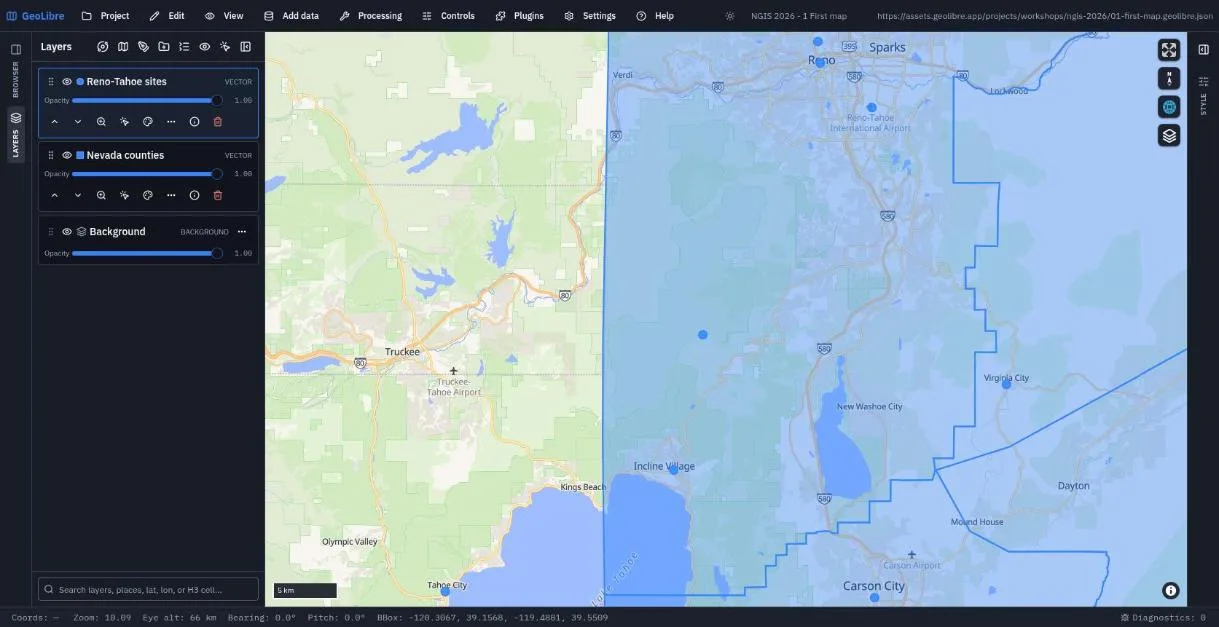
Exercise 1.5: Reopen a project from a link (5 min)
A project file on any public web server opens with one link. Try the finished project for this section:
https://web.geolibre.app/?url=https://assets.geolibre.app/projects/workshops/ngis-2026/01-first-map.geolibre.json
You can also use Project → Open from → URL... inside the app, or Project → Open from → File... for the file you just saved.
Check your work
Going further
- Open Help and browse the keyboard shortcuts and the command palette.
- Switch the engine under View → Rendering engine to Cesium and back.
- Read Interface Overview and Projects.
Break: 8:50 - 9:00. Next: 2. Accessing Cloud-Hosted Vector Data