4. Attributes, Editing, and Spatial SQL
11:00 a.m. - 12:00 p.m.
Lecture 10 min · Hands-on 40 min · Break 11:50 - 12:00, then lunch until 1:00
Learning goals
By the end of this section you will be able to:
- Read a layer's attribute table: sort, search, profile every column, and chart a field before you style or filter by it.
- Derive new fields with the field calculator, including geodesic areas that are real square kilometers even though the data is in longitude and latitude.
- Build a selection four ways (by expression, by location, by drawing, by clicking rows) and summarize just the selected features.
- Tell a selection from a filter, and use expression filters and quick filters.
- Query map layers and remote files with DuckDB spatial SQL in the browser, and keep a query as a live layer that re-runs on refresh.
- Digitize a polygon, turn it into an editable layer, add and edit attributes, and use it in a spatial selection.
Lecture (10 min)
Every map is a view of a table
Sections 1 to 3 treated layers as pictures. This section opens the table underneath. Three ideas carry through every exercise:
- One selection, shared everywhere. The attribute table and the map hold the same selection. Rows you click highlight on the map; features you pick on the map scroll the table. Field statistics, the field calculator, and export can all be limited to that selection.
- A selection highlights; a filter hides. A selection is a temporary set you act on. A filter is a persistent rule saved with the project that stops non-matching features from drawing, like an ArcGIS definition query. Neither changes the data.
- Everything runs in your browser. The attribute table, the expression engine, the field calculator, and three spatial SQL engines all run on your laptop. There is no database to install and no server to connect to.
The attribute table
Open it from Layer actions (⋯) → Open attribute table. It docks below the map. Rows are virtualized, so there is no paging and no row limit: sorting, searching, and every dialog work on all the rows in memory, not just the ones on screen. The toolbar holds the tools for the rest of this section:
| Button | What it does |
|---|---|
| Edit attribute values / Save attribute edits | Turn cells into inputs, then commit the edits to the layer |
| Add field | A new Text, Number, or Boolean column with an optional default |
| Calculate field values from an expression | The field calculator: update a field or create one |
| Manage fields | Rename, hide, reorder, delete, or exclude fields from export |
| Explore all fields at a glance | The column explorer: type, nulls, distinct values, distribution |
| Field statistics | Count, nulls, unique, min, max, mean, median, standard deviation, sum, for all, filtered, or selected features |
| Charts | Histogram, scatter, bar, line, box plot, or pie, downloadable as PNG or SVG |
| Export selected layer | GeoJSON, GeoParquet, GeoPackage, KML, KMZ, zipped Shapefile, or CSV |
Look at the distribution before you classify. A histogram tells you whether a field is skewed, bimodal, or full of nulls, which decides the classification scheme in Section 3 and the thresholds you pick here.
Degrees are not meters
GeoLibre reprojects vector layers to WGS84 (EPSG:4326) on load. A planar area on those coordinates is in square degrees, which is fine for ranking and meaningless as a measurement, and a degree of longitude shrinks as you move north. GeoLibre gives you two ways to get real units:
- The field calculator's
$area(unit),$length(unit), and$perimeter(unit)are geodesic: computed on the WGS84 ellipsoid, in square meters, square kilometers, hectares, acres, and more. No reprojection needed. - In SQL, DuckDB's
ST_Areais planar (square degrees). ItsST_Area_Spheroidis ellipsoidal but expects latitude, longitude axis order, so wrap the geometry inST_FlipCoordinatesfirst. Exercise 4.6 shows what happens when you forget.
Four ways to select
| Method | Where | Best when |
|---|---|---|
| By clicking | Rows in the table (Ctrl/Cmd-click toggles, Shift-click a range) |
You are looking at the rows |
| By drawing | Layer actions → Select features (click, rectangle, polygon, freehand, radius) | You can see the features on the map |
| By expression | Layer actions → Select by expression… | The rule is about attributes |
| By location | Layer actions → Select by location… | The rule is about another layer (intersects, is within, contains, is disjoint) |
Each dialog has Modify current selection by: create a new selection, add to it, remove from it, or select within it. Chaining these is how compound questions get answered without intermediate layers.
Expressions use MapLibre expression syntax, JSON arrays such as
[">=", ["get", "mag"], 4], because they compile straight into the renderer.
The Expression builder… button next to every expression box lists the
functions and fields and previews the result on real features. The field
calculator is the one exception: it has its own compact syntax, such as
round(AWATER / (ALAND + AWATER) * 100, 1).
Three SQL engines in the page
Processing → SQL workspace docks an editor and a results grid below the
map. Every vector layer on the map is a table, with its geometry in a column
named geom.
| Engine | Use it for |
|---|---|
| DuckDB (default) | Almost everything. The only engine that reads remote files and URLs directly, and the only one that makes live query layers |
| PostGIS (PGlite) | Running an existing PostGIS query unchanged. About a 19 MB download on first use |
| Apache Sedona | Sedona SQL. The in-browser build cannot reference attributes by name |
A result with a geometry column can go on the map two ways. Add as layer adds a snapshot. Add as query layer keeps the SQL with the layer: Layer actions → Refresh re-runs it, and Edit query in SQL workspace reopens it. That is the closest GeoLibre gets to a database view.
Coming from QGIS or ArcGIS
The attribute table, field calculator, Select by Expression, and Select by Location work the way they do in QGIS and ArcGIS Pro. The SQL workspace is closest to QGIS's DB Manager with virtual layers, except there is no database: the engines run in the page over the layers you already have. Editing is two steps, as in ArcGIS: Save attribute edits commits to the layer in GeoLibre, and a separate Save edits to … command (desktop app, ArcGIS services) writes back to the source.
Hands-on (40 min)
Start a new project: Project → New…, set Project name to
NGIS 2026 - 4 Attributes, editing, and SQL, pick the Positron basemap,
and click Create. Then choose Add data → Vector layer and load these
three URLs (paste each into the URL box and click Load):
https://data.source.coop/opengeos/data/workshops/ngis-2026/nv_counties.geojson
https://data.source.coop/opengeos/data/workshops/ngis-2026/nv_earthquakes.parquet
https://data.source.coop/opengeos/data/workshops/ngis-2026/reno_sites.geojson
Close the Add Vector Layer panel with its ×. The Layers panel lists
reno_sites, nv_earthquakes, and nv_counties. The earthquakes come from
GeoParquet this time, so mag and depth arrive as real numbers instead
of the text a CSV produces.
Exercise 4.1: Read the table before you touch it (5 min)
- On the
nv_earthquakesrow, open Layer actions (⋯) → Open attribute table. The footer reads 8031 features. - Click the
magcolumn header twice to sort descending. The top three rows are the M7.1 Ridgecrest Earthquake Sequence (California, July 2019), the M6.5 Monte Cristo Range, NV Earthquake (May 2020), and the M6.4 Ridgecrest foreshock. - Type
Minainto Search attributes…. The footer changes to 8031 features · 1547 shown: one event in five is described relative to the small town of Mina, near the Monte Cristo Range. Clear the search box. - Click Explore all fields at a glance. The column explorer profiles all
eight fields at once. Note:
mag: minimum 2.5, mean 2.9494, maximum 7.1.magType: 8 unique values and 1 null.ml(local magnitude) accounts for 6,497 events,mdfor 894,mwfor 369.depth: minimum -3.37. A negative depth is an event located above sea level, which happens in mountains when depth is measured from the geoid.
- Close the explorer and click Charts. Set Chart type to
Histogram, Field to
mag, and Bins to20. The first bar, magnitudes just above 2.5, holds about 3,290 events, and the bars fall off steeply after that.

Discussion
With a distribution this skewed, what would five equal interval
classes on mag look like on a map? Which scheme from Section 3 would
you choose instead?
Close the chart.
Exercise 4.2: Calculate fields, in real units (5 min)
- Close the earthquake table. Open Layer actions → Open attribute table
on
nv_counties. It has 17 rows and the Census fieldsGEOID,NAME,NAMELSAD,ALAND(land area in square meters), andAWATER(water area). - Click Calculate field values from an expression. Set the first menu to
Create field, type
area_km2as the new field name, and set Output type to Number. -
Under Geometry, keep Area, choose km², and click Insert. The expression becomes
$area("square-kilometers"). Wrap it so it reads:round($area("square-kilometers"))The Preview shows 23039 for the first county, White Pine. 4. Click Calculate, then sort
area_km2descending. Nye tops the list at 47,129 km², then Elko (44,552) and Lincoln (27,547). 5. Check the result against the Census: Nye'sALANDplusAWATERis 47,134,147,195 m², or 47,134 km². The geodesic area from the polygon agrees to about 0.01%. 6. Run the calculator again: Create fieldwater_pct, Output type Number, expression:round(AWATER / (ALAND + AWATER) * 100, 1) -
Sort
water_pctdescending. Carson City leads at 8 percent, then Douglas (3.8) and Washoe (3.4). All three border Lake Tahoe.
Calculated fields on a URL layer are kept only if you embed them
nv_counties was loaded from a URL, so the project normally stores the
URL, not a copy of the data. Once you edit its attributes, Project →
Save asks Embed edited vector data? Click Embed data and the 17
counties, with area_km2 and water_pct, are written into the project
file (about 86 KB). Save without data keeps only the URL, and the
fields are gone when you reopen it. A virtual field (Style panel →
Virtual fields) or a SQL query (Exercise 4.7) keeps derived values
without copying the data.
Exercise 4.3: Select by expression and summarize the selection (4 min)
- Close the county table and open the earthquakes table again (Layer
actions → Open attribute table on
nv_earthquakes). Open it first: opening the table after you select clears the selection. In the table toolbar, tick Zoom to selection. -
On the
nv_earthquakesrow, open Layer actions → Select by expression…. Select features from already readsnv_earthquakes. Type this into Expression:[">=", ["get", "mag"], 4] -
Click Select features. The dialog reports 262 of 8031 feature(s) selected (262 matched). The table footer reads 262 selected, the selected points turn yellow, and the map zooms out to frame all 262 events.
- Close the dialog with its ×. The selection stays.
- Click Field statistics. Set Field to
magand Scope to Selected (262). The summary reads: count 262, min 4, max 7.1, mean 4.4317, median 4.3. Switch Scope back to All features (8,031) and compare: the mean drops to 2.9494.

Exercise 4.4: Select by location, within the selection (3 min)
The extract includes events in California. Which of the 262 strong events were in Nevada?
- Keep the selection. Open Layer actions → Select by location… on
nv_earthquakes. - Set Where the feature to Is within, By comparing to the features
of to
nv_counties, and Modify current selection by to Selecting within the current selection. - Click Select features. The dialog reports 101 of 8031 feature(s) selected (2827 matched). 2,827 events in total fall inside a Nevada county; 101 of them are M4 or more.
- In the table, set the Feature view menu to Show selected (101) to list only those rows. Set it back to Show all features, then click Clear selection.
Discussion
Select by location answers which ones. A spatial join answers what do they inherit, such as each earthquake's county name. If you ran a spatial join and then deleted the rows without a match, which tool did you actually want?
Exercise 4.5: Filters hide, selections highlight (4 min)
- Open Select by expression… on
nv_earthquakesagain. The expression from Exercise 4.3 is still there. - Click Filter layer instead of Select features. The dialog reports Layer filter applied: 262 of 8031 feature(s) match. The small events disappear from the map, and a funnel icon appears on the layer row: A persistent filter is hiding some of this layer's features.
- Click Clear layer filter and close the dialog. All 8,031 points return.
- Open the Style panel for
nv_earthquakes(the palette icon on its row) and scroll to Quick filters. Click Add a filter… and choosemag. A range slider appears with Minimum and Maximum boxes (2.5 to 7.1). - Type
5into Minimum and pressTab. Only the largest events remain, and the funnel icon now reads A quick filter is hiding some of this layer's features. - Click Remove the filter on mag to drop it.
Filters compose
Quick filters, expression filters, a Time Slider window (Section 6), and
rule-based symbology all combine instead of replacing each other. Filters
hide features on the map only. They do not narrow the attribute table or
change the selection. A quick filter on a text field such as magType
offers a Values list of checkboxes instead of a range, each with its
count across the whole layer: ml 6,497, md 894, mw 369, and mlr
246 of the 8,031 events.
Exercise 4.6: Spatial SQL, and a degrees-versus-meters trap (6 min)
- Close the Style panel. Choose Processing → SQL workspace. It docks below
the map with Engine: DuckDB. The Queryable layers line lists
nv_counties,nv_earthquakes, andreno_sites. -
Replace the sample query with the one below and press
Ctrl+Enter(Cmd+Enteron macOS), or click Run:DESCRIBE nv_earthquakes;geomisGEOMETRY('EPSG:4326')andtimeis aBIGINT: milliseconds since 1970, as the USGS publishes it. 3. Find the ten strongest events, with a readable date:SELECT place, mag, depth, strftime(epoch_ms(time), '%Y-%m-%d') AS date FROM nv_earthquakes ORDER BY mag DESC LIMIT 10;The first rows are Ridgecrest (7.1, 2019-07-06), Monte Cristo Range (6.5, 2020-05-15), and Ridgecrest again (6.4, 2019-07-04). Note the 2024 Parker Butte, Nevada Earthquake (M5.71, 2024-12-09) in sixth place. 4. Now compare three ways to measure county area:
SELECT NAME,
       round(ST_Area(geom), 3) AS area_deg2,
       round(ST_Area_Spheroid(geom) / 1e6) AS wrong_km2,
       round(ST_Area_Spheroid(ST_FlipCoordinates(geom)) / 1e6) AS area_km2
FROM nv_counties
ORDER BY area_km2 DESC
LIMIT 5;
NAME area_deg2 wrong_km2 area_km2 Nye 4.837 NaN 47129 Elko 4.779 NaN 44552 Lincoln 2.813 NaN 27547 ST_Areareturns square degrees.ST_Area_Spheroidon the raw geometry returnsNaN, because it reads the first coordinate as latitude and Nevada's longitudes (about -117) are not valid latitudes. WithST_FlipCoordinates, the SQL area matches the field calculator's 47,129 km² exactly.
Discussion
Elko and Nye differ by only 1% in square degrees but by 6% in square kilometers. Why? (Hint: which county is farther north?)
Exercise 4.7: Earthquakes per county as a live query layer (7 min)
-
Run the spatial join. It counts earthquakes inside each county, keeps the county geometry, and computes a density per 1,000 km² with a real area:
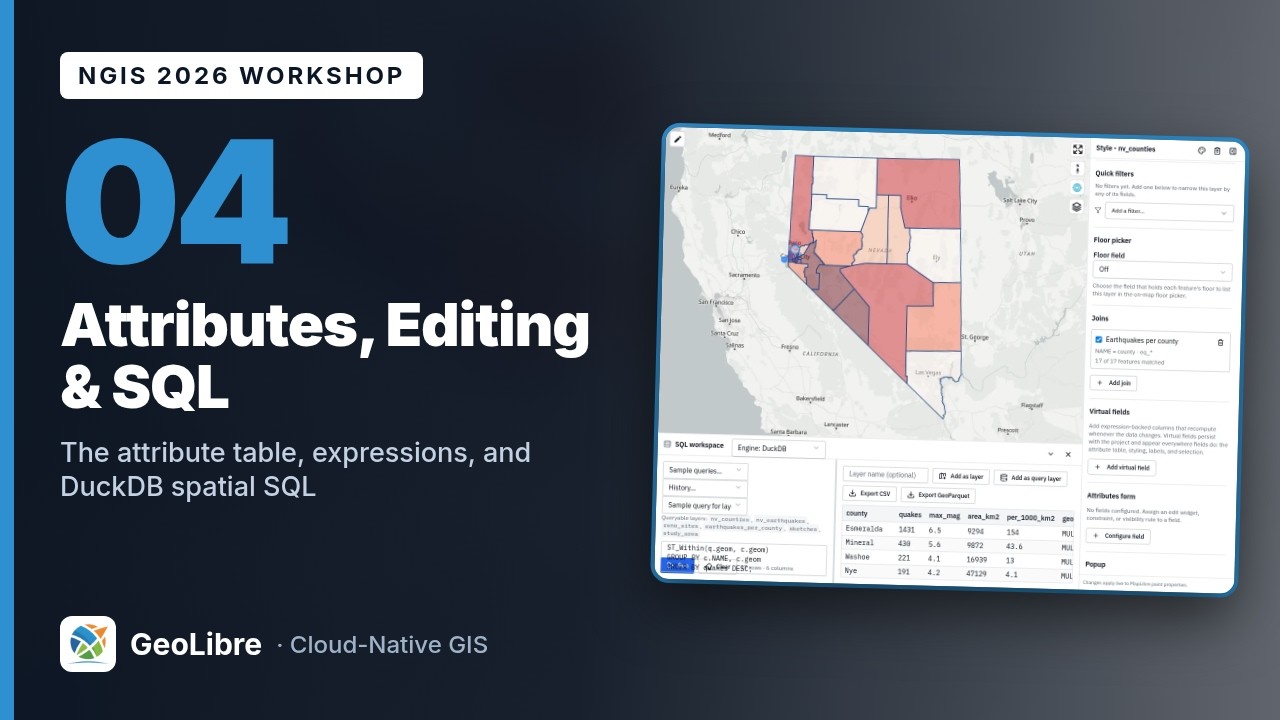
SELECT c.NAME AS county, count(q.id) AS quakes, round(max(q.mag), 1) AS max_mag, round(ST_Area_Spheroid(ST_FlipCoordinates(c.geom)) / 1e6) AS area_km2, round(count(q.id) * 1000 / (ST_Area_Spheroid(ST_FlipCoordinates(c.geom)) / 1e6), 1) AS per_1000_km2, c.geom FROM nv_counties c LEFT JOIN nv_earthquakes q ON ST_Within(q.geom, c.geom) GROUP BY c.NAME, c.geom ORDER BY quakes DESC; -
The result has 17 rows. Esmeralda leads with 1,431 events, a maximum of M6.5, and 154 events per 1,000 km²: the Monte Cristo Range sequence. Mineral (430) and Washoe (221) follow. Carson City has only 8 events but, at 407 km², a density of 19.7.
- Type
Earthquakes per countyin the Layer name box above the results and click Add as query layer. The workspace confirms: Added 17 features to the map as query layer "Earthquakes per county". Refresh it from the Layers panel to re-run the SQL. - Close the SQL workspace. Open the Style panel for
Earthquakes per county, set Style type to Graduated, Attribute toper_1000_km2, Scheme to Quantile, click the Colormap button and choose Reds, then click Apply style type. The class breaks read about 0.7, 1.42, 2.38, and 3.82. - Hide
nv_countiesandnv_earthquakesto see the choropleth. - Open Layer actions on
Earthquakes per county. Note Refresh (re-run the SQL against the current layers; the row then reads Refreshed 17 features.) and Edit query in SQL workspace (reopen the statement).

Discussion
The 17 county counts add up to 2,827, the same number Select by location
matched in Exercise 4.4, yet the layer holds 8,031 events. Which part of
the query removed the other 5,204? Why does the query use LEFT JOIN
instead of JOIN?
Keep the geometry column
A result can become a map layer only if it carries geometry. Leave c.geom
out of the SELECT list and Add as layer has nothing to draw. While
you iterate on a query, add LIMIT 10; GeoLibre also asks before turning
more than 500,000 rows into features.
Exercise 4.8: Digitize a study area and edit its attributes (6 min)
- Zoom in to Reno and Sparks: type
Renoin the search box and pick Reno, Washoe County, Nevada, United States under Places (matches from your own layers are listed first). The map frames Reno and Sparks. Shownv_earthquakesagain. - Click the GeoEditor button in the Layers panel toolbar (the pen icon). The editing toolbar opens on the left edge of the map.
- Click the Polygon tool (the first button). Click four or five points on the map to draw a box about 9 km across at the south end of the Truckee Meadows, from just south of the Reno-Tahoe airport down toward Steamboat, east of I-580. Click the first point again to close the shape. Few M2.5+ events fall in downtown Reno or Sparks, so a box drawn there selects none.
- A Feature properties panel asks for Height (m). Leave it empty and click Save. A Sketches layer appears at the top of the Layers panel. Close the editing toolbar with its ×.
- Sketches belong to the editor. To make an ordinary layer you can edit, open
Layer actions → Export Sketches as new layer → Clear Sketches after
export. A Sketches export layer appears. Double-click its name and
rename it
Study area. - Open Select by location… on
nv_earthquakes: Is within,Study area, Creating a new selection. Click Select features. The count depends on the polygon you drew; a box over the south Truckee Meadows selects about a dozen events (11 in the instructor's run). - Open the attribute table for
Study area. Click Add field, typenameas Field name, keep Type Text, and click Add field. - Click Calculate field values from an expression: Create field
area_km2, expressionround($area("square-kilometers"), 1). The preview shows your polygon's area (85.5 km² for the instructor's box). Click Calculate; the table gains anarea_km2column. - Click Edit attribute values (the pencil). Type a name such as
East Truckee Meadowsinto thenamecell and click Save attribute edits.

Unlike the URL layers, the study area is saved with the project
A drawn layer has no source URL, so GeoLibre embeds its features, and its
name and area_km2 values, in the .geolibre project file.
Save the project with Project → Save (Ctrl+S, Cmd+S on macOS). When
GeoLibre asks Embed edited vector data?, click Embed data to keep the
county fields from Exercise 4.2.
Bonus 4.9: Join the counts back to the counties (if you finish early)
A join attaches columns from another layer or table by a shared key, and the link stays live: when the joined layer changes, the columns update.
- Open the Style panel for
nv_countiesand scroll to Joins. Click Add join. - Join layer:
Earthquakes per county. Join field:county. Target field:NAME. Field name prefix:eq_. Leave all four Fields to join ticked and click Add. - The join card reads NAME = county · eq_* and 17 of 17 features
matched. Open the county attribute table: new columns
eq_quakes,eq_max_mag,eq_area_km2, andeq_per_1000_km2sit at the right.
Joins are left joins (every county is kept), compare keys as text, and are saved with the project, so this one survives a reload even though the calculated fields from Exercise 4.2 do not.
Bonus 4.10: Query a file you never added to the map
DuckDB reads files by URL, using HTTP range requests, without loading them as layers. Ask the national counties GeoParquet file a question:
SELECT STUSPS, count(*) AS counties, round(sum(ALAND) / 1e6) AS land_km2
FROM 'https://data.source.coop/opengeos/data/workshops/ngis-2026/us_counties.parquet'
WHERE STUSPS IN ('NV', 'CA', 'OR', 'ID', 'UT', 'AZ')
GROUP BY STUSPS
ORDER BY counties DESC;
California has 58 counties, Nevada 17, and Arizona 15, although Nevada's land
area (284,537 km²) is close to Arizona's (294,366 km²). Run
DESCRIBE SELECT * FROM '<url>' first whenever you do not know a file's
columns; here the geometry column is called geometry, not geom.
Bonus 4.11: An attribute form with editor tracking
Forms make bad values hard to type, and editor tracking records who changed what.
- In the
Study areaattribute table, Add fieldstatus(Text). - Open the Style panel for
Study area. Under Editor tracking, tick Track edits on this layer and type your name into Your name (it defaults tolocal-user). Four columns join the table:created_by,created_at,edited_by, andedited_at. -
Under Attributes form, click Configure field. Field:
status. Edit widget: Value map. Tick Required. In Value map entries, type one entry per line:draft=Draft reviewed=Reviewed final=FinalClick Save. The card reads status · Value map · required. 4. Click Edit attribute values in the table. The
statuscell is now a dropdown of Draft, Reviewed, and Final. Choose Reviewed and click Save attribute edits.edited_byfills in with your name andedited_atwith the time.
Then try Processing → GeoLibre toolbox → Vector → Check validity on
nv_counties with the Client (Turf.js) engine. It reports Checked 17
feature(s): 0 invalid. Run a validity check before any overlay: an invalid
polygon can draw perfectly and still make an overlay return nothing.
Check your work
The finished project,
04-attributes-editing-sql.geolibre.json,
restores the Earthquakes per county query layer with its Reds choropleth (use
Layer actions → Refresh to re-run its SQL), the Study area polygon with
its attributes, and the join from Bonus 4.9. As the warning in Exercise 4.2
explains, the area_km2 and water_pct fields calculated on nv_counties are
kept only when you embed the edited data; the finished project was saved
without them, so it stays small and reads the counties from their URL.
Going further
- Layer actions → Select features offers QGIS-style selection by click, rectangle, polygon, freehand, and radius.
- The Edit menu has Invert selection and Export selected features as layer, and Layer actions → Export writes a layer to a file. GeoParquet is the best default for reuse; Shapefile field names are capped at 10 characters.
- Manage fields (or a column header's ⋯ menu) hides fields and marks them Exclude field on export, so a shared file carries only the columns you meant to share.
- Processing → GeoLibre toolbox → Vector has Fix geometries, Check topology rules, and Fix topology next to Check validity, plus Spatial join, Attribute join, and Select by value, which write new layers instead of selections.
- Processing → GeoLibre toolbox → Spatial statistics → Composite score (suitability index) builds a weighted suitability index from several numeric fields.
-
Switch the SQL workspace engine to PostGIS (the first run downloads the engine) and port the join from Exercise 4.7. In PostgreSQL, quote mixed-case columns, cast before rounding, and use a
geographycast for real areas:SELECT c."NAME" AS county, count(q.id) AS quakes, round(max(q.mag)::numeric, 1) AS max_mag, round((ST_Area(c.geom::geography) / 1e6)::numeric) AS area_km2 FROM nv_counties c LEFT JOIN nv_earthquakes q ON ST_Within(q.geom, c.geom) GROUP BY c."NAME", c.geom ORDER BY quakes DESC;Esmeralda again returns 1,431 events and 9,294 km². - Add data → ArcGIS layer adds an ArcGIS Feature Service. Services that allow editing get Layer actions → Save edits to ArcGIS service, which writes your edits back through
applyEditsand respects the service's domains and subtypes. - Read Attribute Table, SQL Workspace, Spatial SQL, and Layers.
Break: 11:50 - 12:00. Lunch: 12:00 - 1:00. Next: 5. Analysis and Processing